SCFQFT
SCF equations
Anomalous Green's function
The spin index can be omitted, since the spin sector can be always block diagonalized.
Dyson equation
where
With ladder approximation, the self energy equation is
Do Fourier
where
The non-diagonal part is actually the order parameter in standard BCS. This may be our starting point?
The Bethe-Salpeter equation
where
is the regularized pair propagator. Note here the is the total momentum of the pair, and is the Bosonic Matsubara frequency, corresponding to the total energy of the pair.
Denote , , then
Decompose Equation 10 into spherical coordinates, we get
In numerics we need to substitute all into
Remark
could be . I would choose to calculate it manually instead of reading from the pre-computed Green function mesh.
in real Space
where is defined as a constant with ultraviolet momentum cutoff .
goes to infinity when .
Remark
This UV divergence only occur in continuous system. In lattice model, the momentum cutoff is naturally chosen as
If we want to compare with results on the Tianyuan Quantum Simulator, what is the suitable model to use?
Arguably I think continuous model might be better, since the spacing of cold atoms are not as uniform as in the real material.
necessary explanation for SCF equations
The Bethe-Salpeter Equation 9 is introduced since we need to describe the two particle correlations.
The third term contains a vertex, we define the vertex as
The node is painted black, meaning it is resummed by irreducible vertex functions.
If we introduce the pair propagator
which is exactly the second column diagram.
The vertex function can be obtained by
where is the irreducible vertex function. or equivalently
This is the Bethe-Salpeter equation.
An approximation we made here is to substitute the irreducible vertex function with
where are the s,t,u channels at tree level.
We will see that Equation 18 leads to a ladder approximation.
The matrix form of pair propagator is
Because of the localization nature of the vertex function, we treat it in the space, where is a constant.
Thus
Remark
These equations include space-time non-homogenous parameters, the number of parameters depends on the discretization of space-time.
Remark
The question is, it will be more clear to discretize in and space, more problematic in real space?
mean-field Green's function
Take the weak coupling limit, . Because , in our unit, , the leading order of Bethe-Salpeter Equation 9 is
Fourier transform the self-energy Equation 5, we get
Thus (because of the orthogonality of the basis functions)
The Fourier transform of self-energy is non-zero only when and .
The , component of the normal green function can be obtained by
Thus
Insert this into the Dyson Equation 3, we get
By Fourier transform of Equation 2, we get
Remark
There is a deduction gap in the inversion procedure. Solve it or ask!
You are believed to reproduce this (with a Bogoliubov transformation of the Nambu spinor I think)
And the anomalous Green's function
where
Scale the equation of with respect to and
Scale invariance
The SCF equations Equation 3 Equation 5 Equation 9 Equation 10 have 3 parameters, temperature (hidden in Matsubara summation), the Fermion density (hidden in the chemical potential in Dyson Equation 3), the coupling strength in Bethe-Salpeter Equation 9.
Because the quadratic energy dispersion and the contact potential (in the context of discrete lattice model, i.e. Hubbard model), the interaction term doesn't depend on relative distance, the SCF equations are scale invariant.
The is of the dimension of energy, transform to real space and imaginary time gives dimension of
Thus we can define dimensionless parameters for SCF equations
Definition 1 Define dimensionless temperature as
Define dimensionless coupling strength as
Symbols of temperature and the renormalized interaction strength are abused in the book. From now on I will only use to represent the temperature.
Remark
However, our SCF equations are derived in the dilute limit where . As the reaches 1 or be much larger than 1, the Pauli blocking will be extremely relevant.
Tuning the coupling strength, we can see the BCS-BEC crossover.
Remark
Assumptions used in SCF equations
- In Equation 18, the irreducible vertex function is replaced by the bare interaction vertex
- The interaction is assumed local in botsh real space and imaginary time.
These assumptions lead to a ladder approximation.
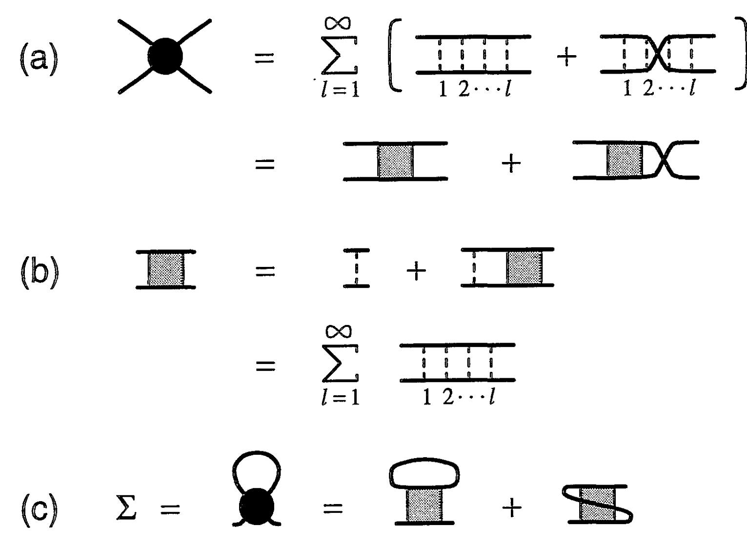
In Figure 1 (a) direct and interchange lattice diagrams are considered
Remark
Why don't we have diagrams including multiple interchange vertex?
I think maybe it's because two channel interaction may go back to the ordinary ladder diagram.
SCF procedure
To study the BCS-BEC crossover region, neither the weak coupling limit nor the strong coupling limit is valid.
We start with inserting the mean-field Green's function Equation 28 Equation 29 into the pair propagator Equation 10, we get (All in the space)
Remark
We used bare vertex to substitute the irreducible vertex. Does it mean the Green function can be also treated freely with this order of approximation?
According to the book, I think the answer is probably NO.
Note on Fourier transform
We use the convention
Definition 1